As we boldly march into our inevitable digital future, the competencies that were once the exclusive domain of business managers are quickly becoming prerequisites for entry-level jobs. Such is the case with the backbone of modern office productivity: the spreadsheet. It's not enough to be a data entry pro. Today's jobseekers need to know how to analyze and manipulate information. It also doesn't hurt to have a nice Chromebook.

SUM is one of the most useful functions in Google Sheets' arsenal, but sometimes you don't want the sum of every number in a range. Sometimes you need to be specific about which numbers you'll add together and which numbers you'll exclude. For the discerning spreadsheet wizard, only SUMIF will do.

How to use SUMIF

To use SUMIF, you need a range of data from which you want to sum values and a criterion by which you want to evaluate whether to include a number in your sum.

Create a simple SUMIF formula

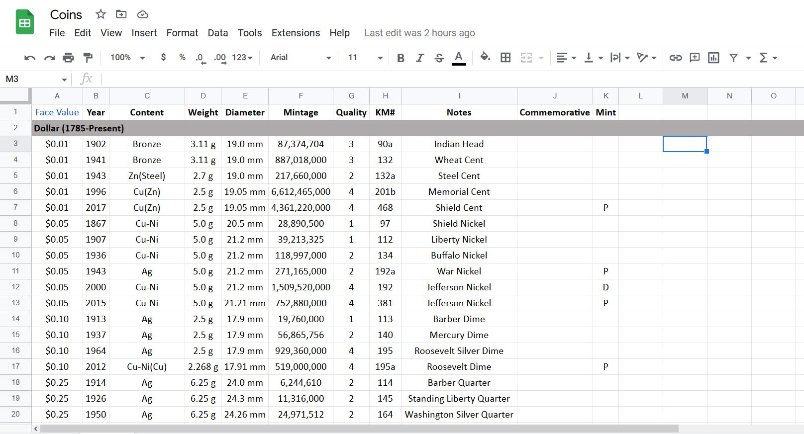
Let's play with a data set to see what this looks like in practice and find the total face value of the quarters in a coin collection.

1. Select the cell into which you want the sum to appear.

   

2. Enter the formula =SUMIF(A3:A191, .25).
3. Press Enter.

   

This is the simplest example of the SUMIF function. Let's take it up a notch.

Sum numbers that match specified criteria

In the previous example, we evaluated the range of numbers from which we took our sum, but the range we check against a criterion and the range from which we produce our sum doesn't have to be the same set of data. Instead, we can indicate one range of data to check against a criterion and another from which to produce our sum. Let's get the total weight of all the coins that contain silver.

1. Select the cell into which you want your sum to appear.
2. Enter the formula =SUMIF(C3:C191, "Ag", D3:D191). The first range (C3:C191) is the range we want to test against the criterion ("Ag"). The second range (D3:D191) is the range from which we want to pull addends for our final sum.
3. Press Enter.

   

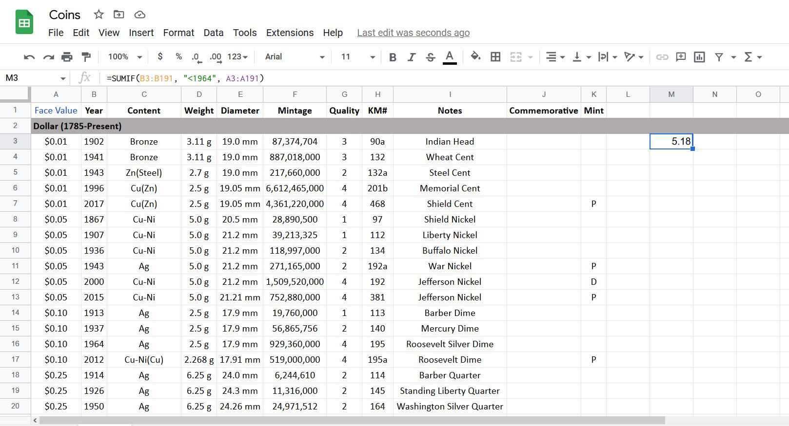
We're doing pretty good, but if you want to flex your spreadsheet muscles around the water cooler, you need to get good with your criteria. So far, we've looked at exact matches, but we can be a bit looser with our inclusion criterion. Let's get the face value of all the coins minted before 1964.

1. Select the cell into which you want your sum to appear.
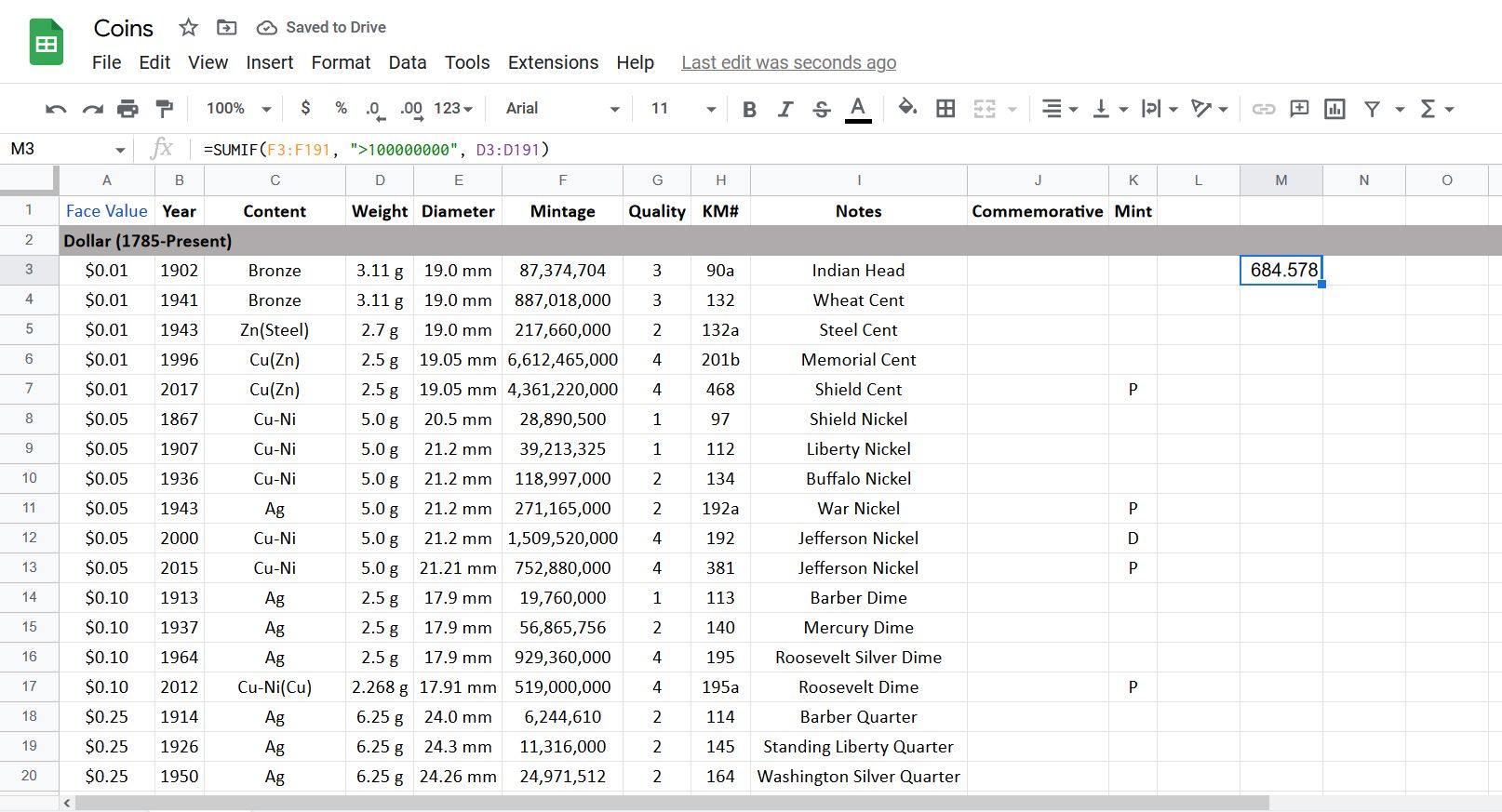
2. Enter the formula =SUMIF(B3:B191, "<1964", A3:A191). Similarly, we could also use the > sign in our criterion. To find the weight of every coin that was part of a mintage of over 100 million, we could use the formula =SUMIF(F3:F191, ">100000000", D3:D191).

   

3. Press Enter.

   

Sum numbers with conditional text criteria

Now that we have a grasp of numbers, it's time for something a bit more tricky: conditional text criteria. Let's find the total face value of all the coins that have any zinc (Zn) in them. If we enter the formula =SUMIF(C3:C191, "Zn", A3:A191) formula, it shows "0" because it's looking for an exact match to the criterion.

The solution to our problem is the asterisk character (*), which is a wildcard input that can stand in for any other character or number of characters. For example, change the criterion to "Zn*" to indicate to Sheets that it should look for "Zn" followed by any combination of zero or more characters. Let's put that in and see what we get.

There seems to be a problem. We can see that there are more coins with zinc, but our formula only shows a total face value of $0.01. The solution is to append another asterisk in front of "Zn" in our criterion to indicate that there could be any number of characters in front of or behind "Zn." As long as "Zn" is in there somewhere, SUMIF will count it.

You can also use the question mark (?) as a wildcard for a single character.

When to use the SUMIF function

There are so many use cases for using the SUMIF function that it would be impossible to list them all. Perhaps you print bespoke phone cases for Pixel phones and want to see your sales for particular zip codes. Maybe you have to calculate the overtime payroll by applying time-and-a-half wages to everyone who works more than 40 hours. The important thing is that you have the tool at your disposal when you need it.

If you've used pivot tables before, this SUMIF stuff might sound familiar. Pivot tables hide the functionality of SUMIF under a layer of abstraction, but you can use it by itself when you don't want to deal with the mental overhead that can come with using pivot tables. And if you need a primer on pivot tables, we have a how-to article for that.