8 Google Sheets tips and tricks guaranteed to make you more productive

Some people use Google Sheets for basic stuff. Some use it for complicated statistical calculations. You may use the app to manage your household budget. We know someone who uses a sheet to track every step they've taken during the year.

Whatever your priorities, Google Sheets offers advanced features that increase data accuracy and help you work faster. You can change themes to make the app visually appealing and automate repeated processes on Android phones, tablets, Chromebooks, and personal computers.

Like most apps in Google Workspace, Google Sheets is cloud-based and allows you to sync your work across your devices. Try these tips to maximize the benefits of using Google Sheets.

What is Google Sheets?

Google Sheets is a free and cloud-based alternative to Microsoft Excel. The spreadsheet program is designed for data entry and has an interface that's fit for business or personal use. You can use the app to create and format special blocks called cells, use functions and formulas to alter and calculate values inside cells, and collaborate with people in real time.

Google Sheets is an online app that saves your work as you go. Your data remains private until you give people access to it, the same way most Workspace applications operate. Sheets is free for personal use and has several business plans. A Google Workspace subscription plan unlocks the business versions of Google's other productivity apps.

Google Sheets has a web app you can use from your browser and a mobile app. Using it on your phone limits its functionality, so it's best used for quick edits and not intense computations.

Freeze columns and rows

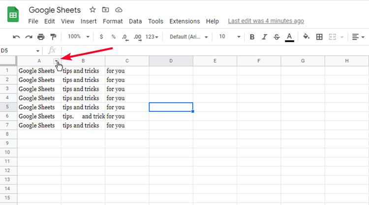
There can be millions of cells in one Google spreadsheet. You could miss important data if you scroll too much. Sheets allows you to freeze columns or rows to ensure that doesn't happen. The frozen cells go along with you when you scroll around the spreadsheet. However, you can't freeze only one cell.

Freeze columns and rows on computers

Click the drop-down arrow beside a column letter.
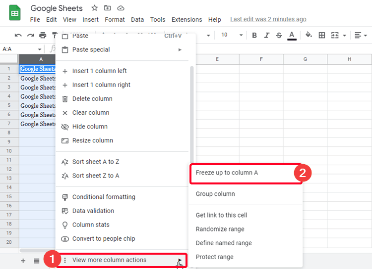
Select View more column actions.
Click the Freeze up to column option.
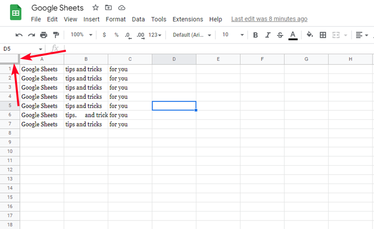
Alternatively, drag the gray bar beside the row numbers to the column you want to freeze.
To freeze columns, drag the bar to the right. To freeze rows, drag the bar down.

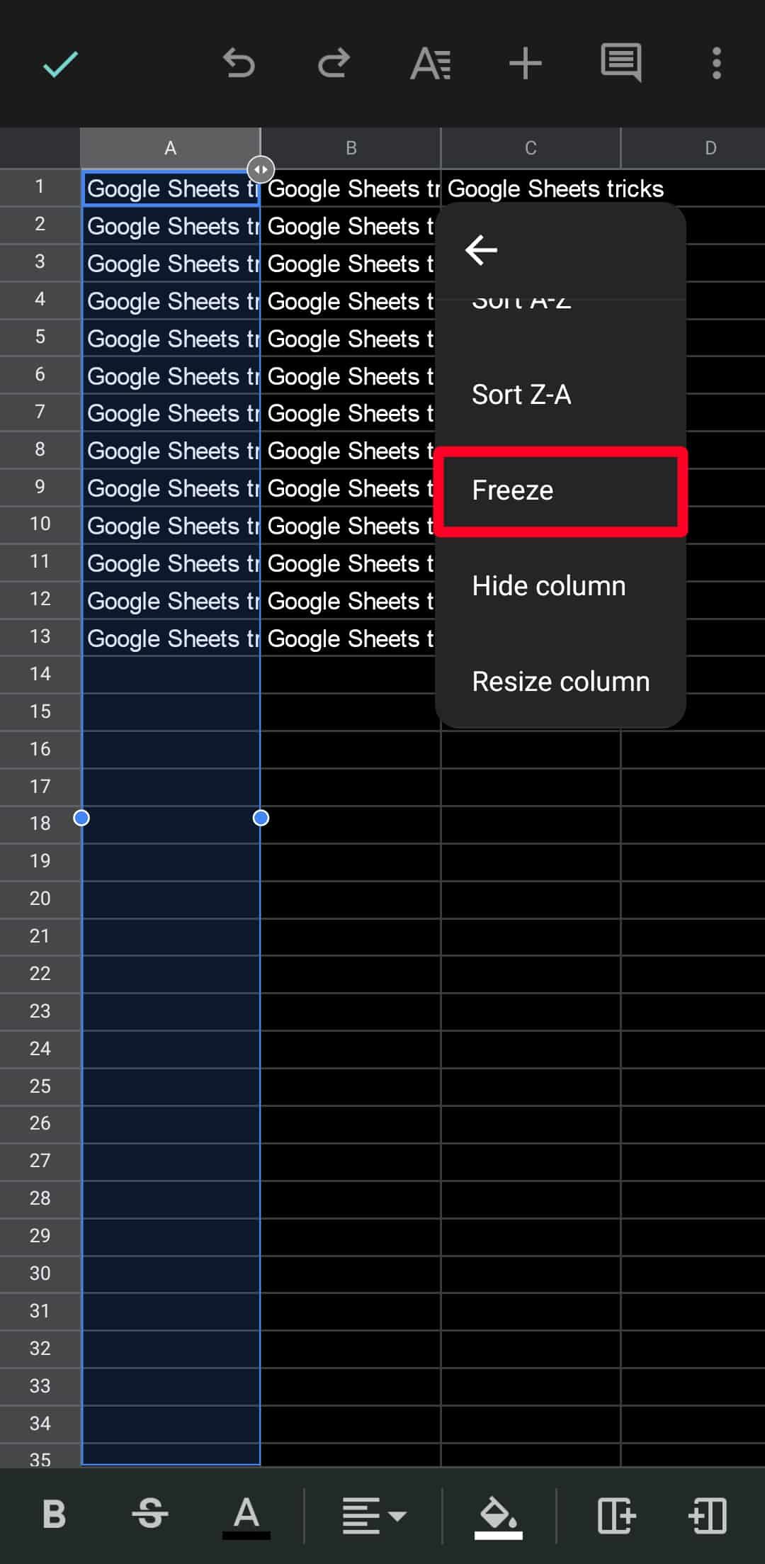
Freeze columns and rows on the mobile app

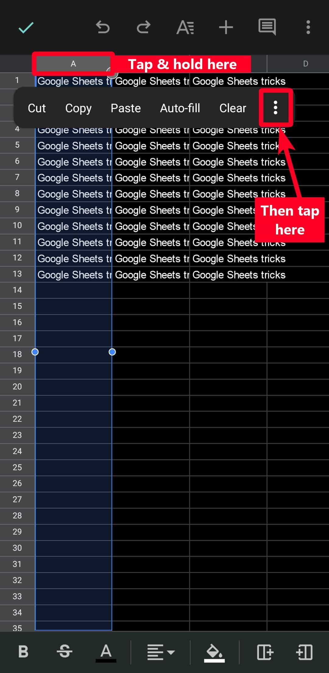
Tap and hold a cell letter. The entire column is highlighted in blue, and a menu pops up. To select an entire row, tap the row number.
Tap the three-dots icon to expand the menu.
Select Freeze.

Filter data

When collaborating with third parties on Google Sheets, your data may combine with theirs and become messy to sort through. The filter option allows you to hide everyone's data and view only yours. Here are the different ways to hide data:

Filter by color: Shows only cells that have colors. You must fill the cells with a unique color or change the text color of their values.
Filter by condition: Limits your spreadsheet view based on specific conditions. For example, to only show cells with values starting with A, B, or C.
Filter by values: Hides specific words or numbers under a column.

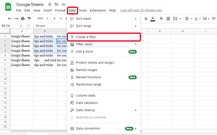
Filter data in Google Sheets on computers

Click a cell that has a value inside it. Double click and drag across columns and rows to select more than one.
Go to Data > Create a filter. Google Sheets automatically places filter icons on the cells.
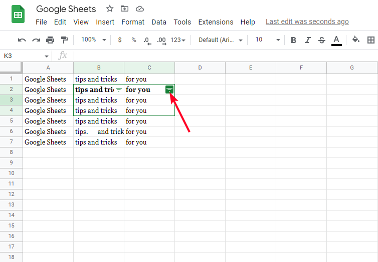
Click the filter icon to choose your filter method.
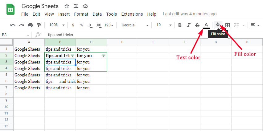
To filter by color, click a cell and use the Fill color button to change its color. Use the Text color button to change the hue of the text.
Click the filter icon and go to Filter by color. Only the colors you chose appear from now on.
To filter by condition, click the filter icon and select Filter by condition.
To filter by values, click the filter icon and uncheck any value from the list. The unchecked values no longer appear in that column.

Filter data in Google Sheets on the mobile app

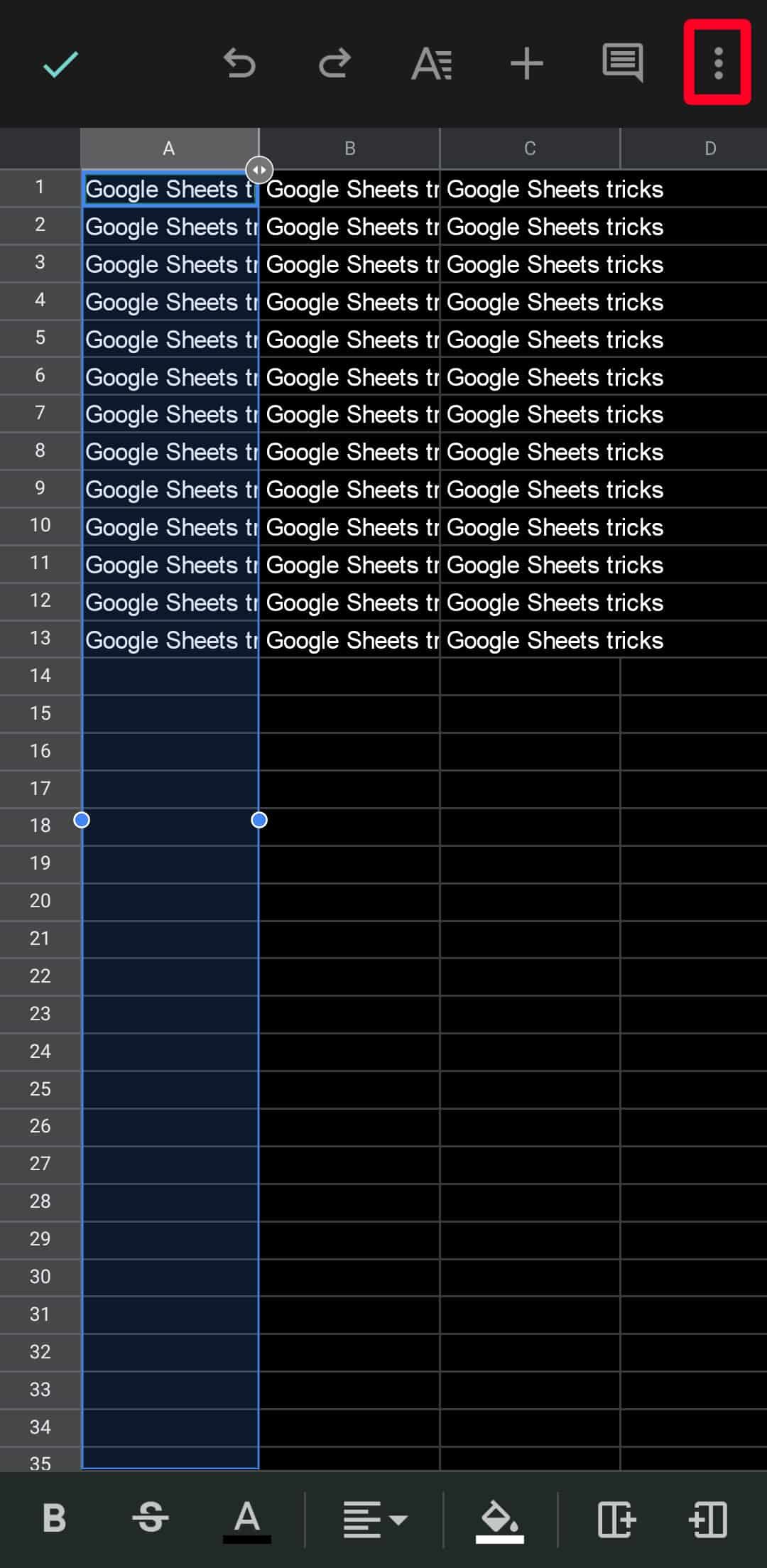
Tap a cell with a value inside it. Tap a cell letter or number to highlight rows and columns.
Tap the three-dot icon to open the sheet's menu.
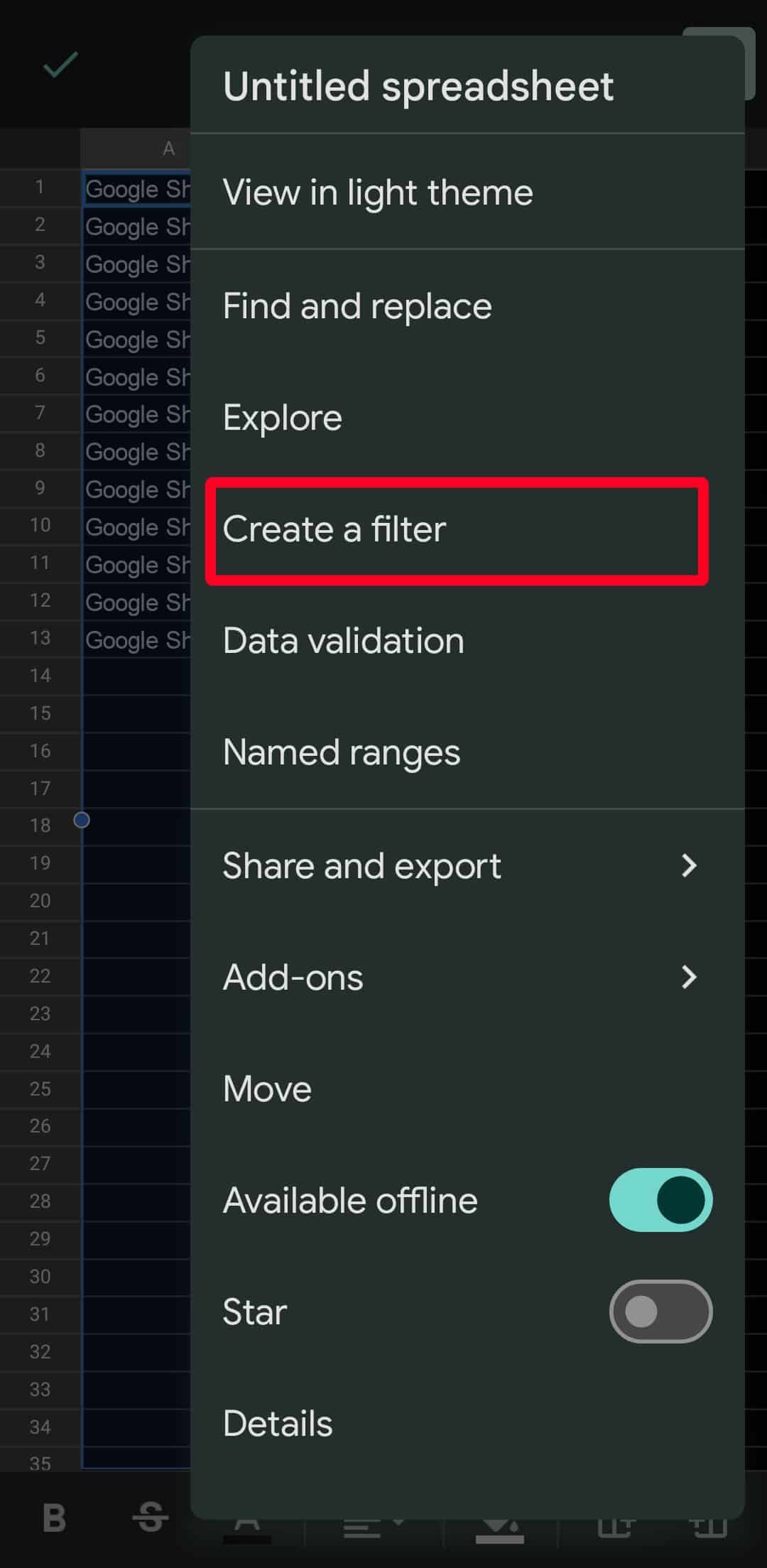
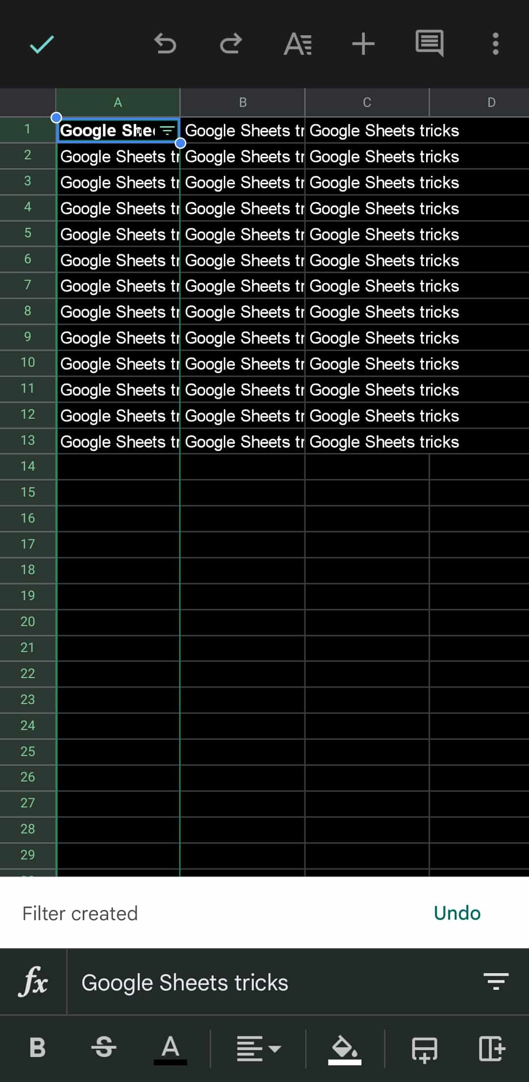
Select Create a filter. A green highlight appears over your selected columns and rows.
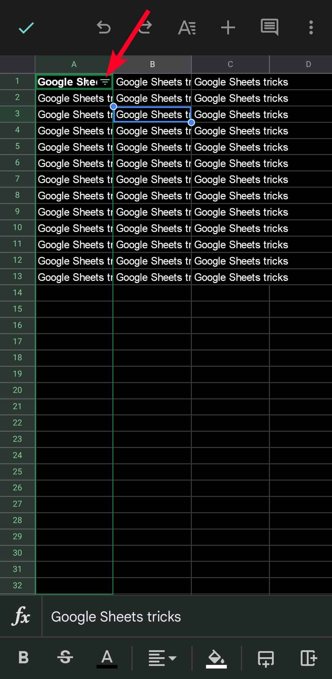
Tap the filter icon. The options for filtering values pop up in a new tab.

Use Google Sheets themes

Google Sheets has 16 themes on the web app. Your theme is set to Standard, but you can change it to a different one. You can customize your selected theme with different fonts and colors for chart backgrounds, text, and hyperlinks.

The theme only applies to the current spreadsheet you're working on, not existing or future spreadsheets. You can only change themes from light to dark on the mobile app, but the theme you choose on the web app reflects on your phone. Use the dark theme to save the battery.

Use Google Sheets themes on computers

Go to Format > Theme. A new sidebar appears.
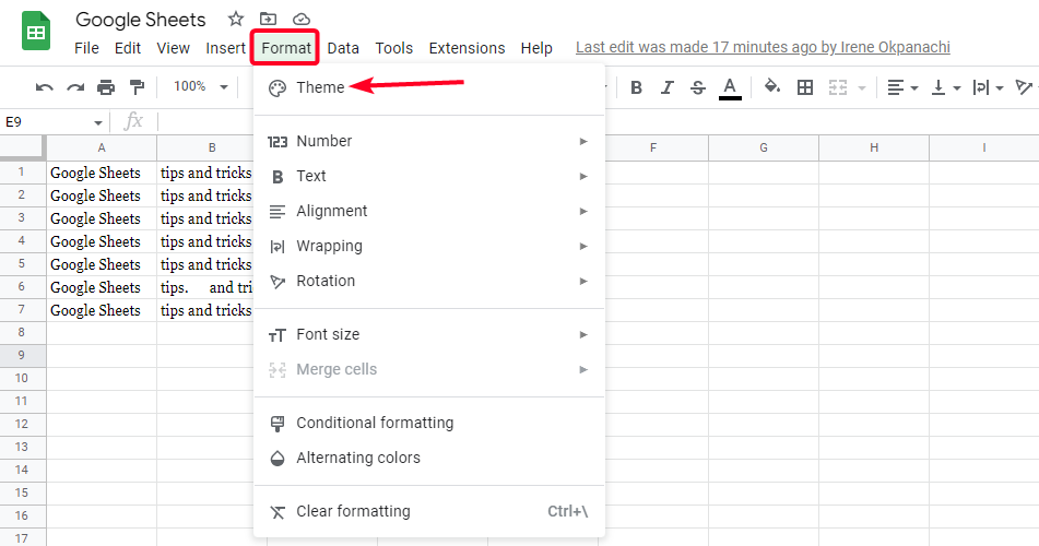
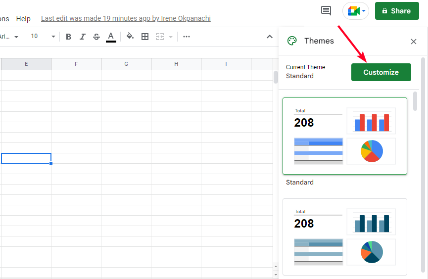
Select a theme from the list.
Click Customize to change the fonts and colors.

Use Google Sheets themes on the mobile app

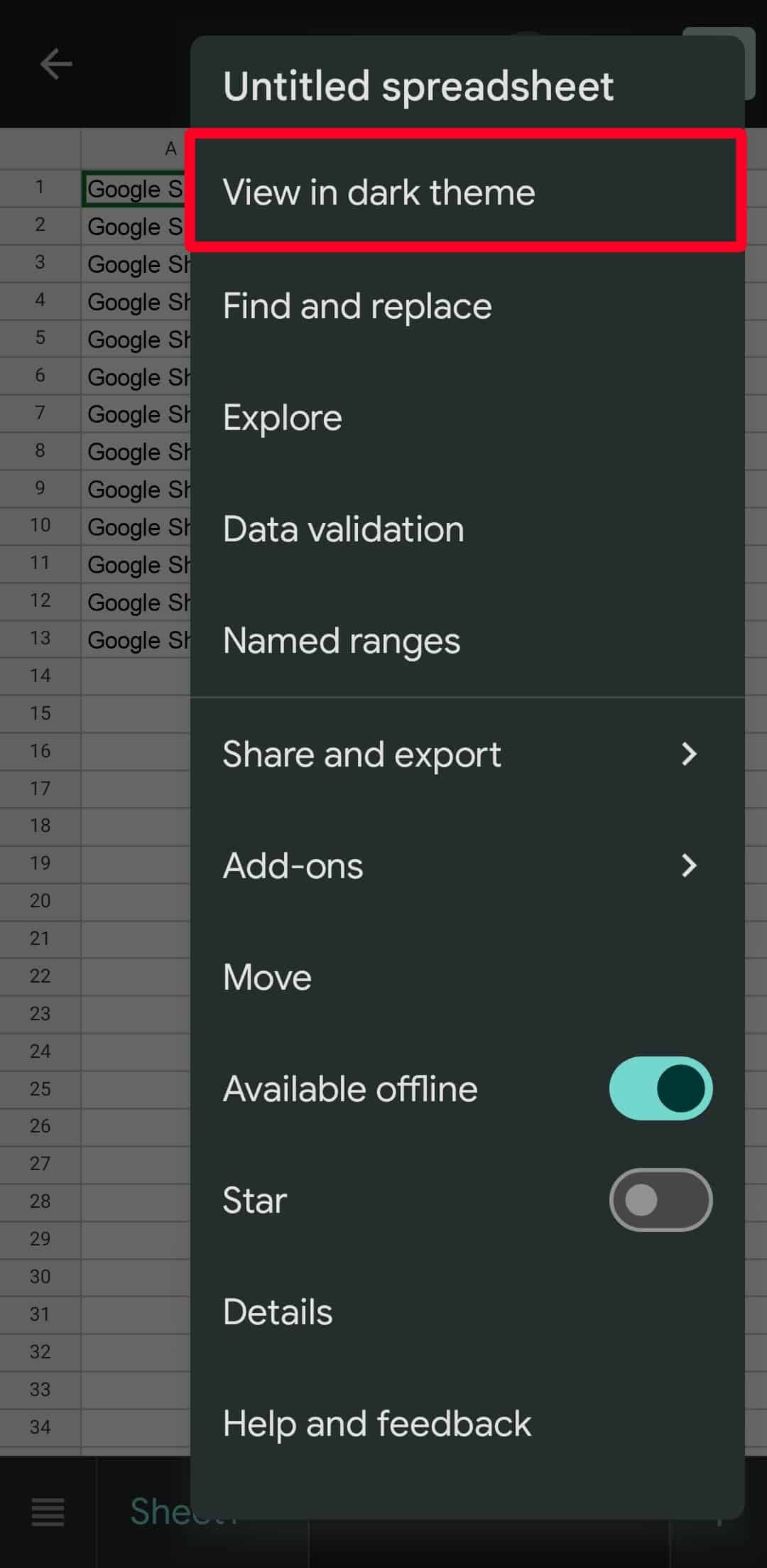
Tap the three-dot icon.
Google Sheets uses your phone's theme settings. If your phone is on light mode, tap View in dark theme to make your spreadsheet's background black.
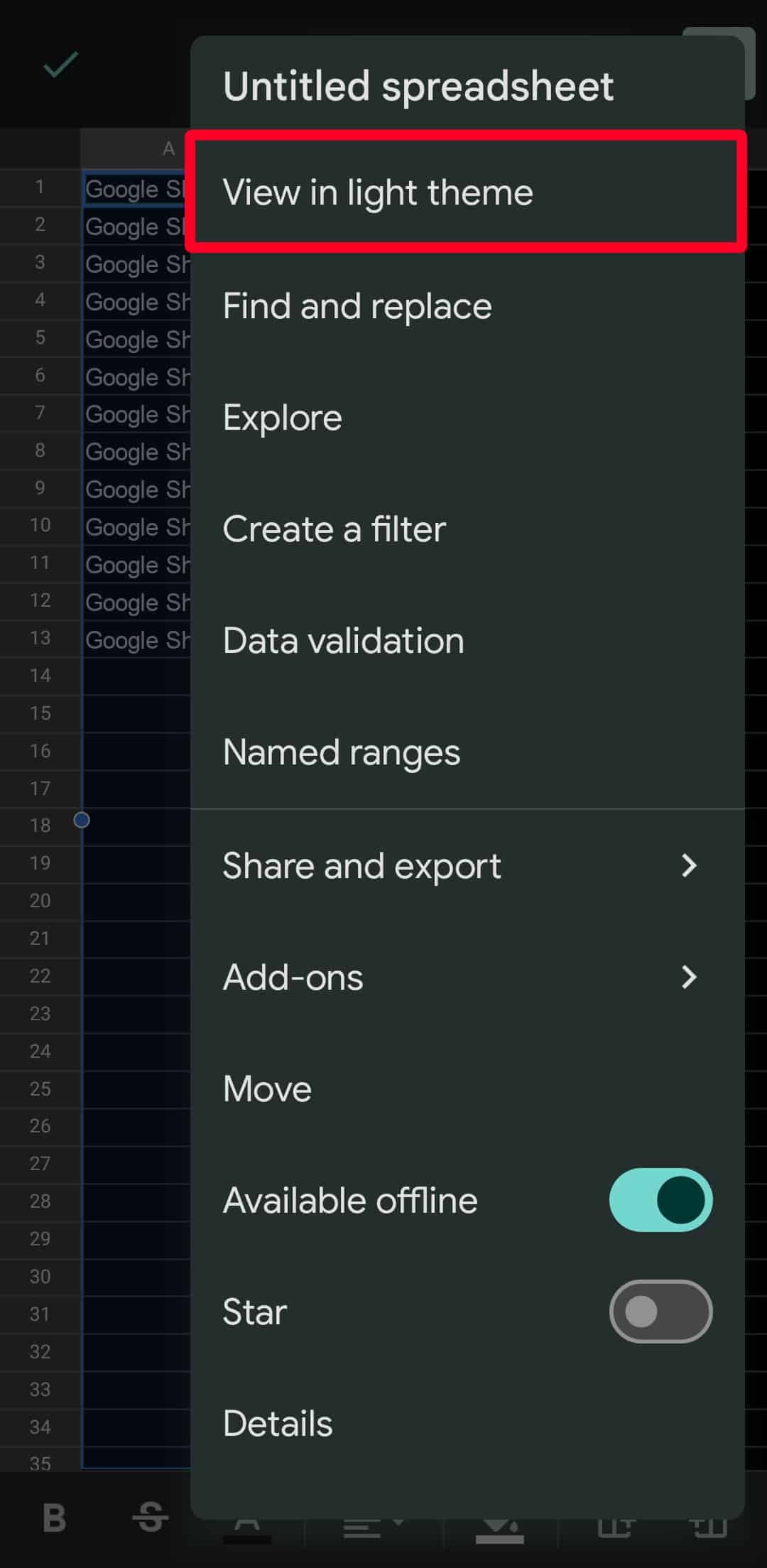
If your phone is in dark mode, tap View in light theme to change the background to white.

Automate repetitive processes

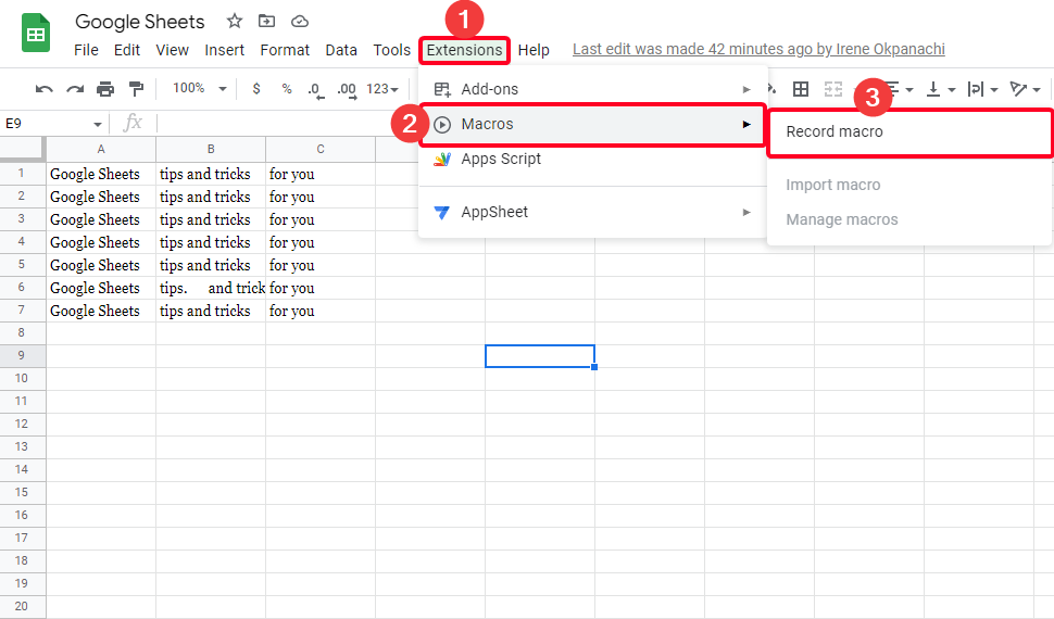
Google Sheets has an extension called Macros. A macro records actions you take on a spreadsheet and then assigns a keyboard command to that set of actions. When you press the command on your keyboard, the recorded action repeats on your spreadsheet. Macros are available on the Google Sheets web app but not the mobile apps. Here are the ways you can use macros:

Use absolute references: Applies your recording to spreadsheets on the same spot in different spreadsheets.
Use relative references: Applies your recordings to any cells you select.

Use Macros from your browser

Go to Extensions > Macros > Record macro.
Macros start recording. Perform any action you need to on your spreadsheet.
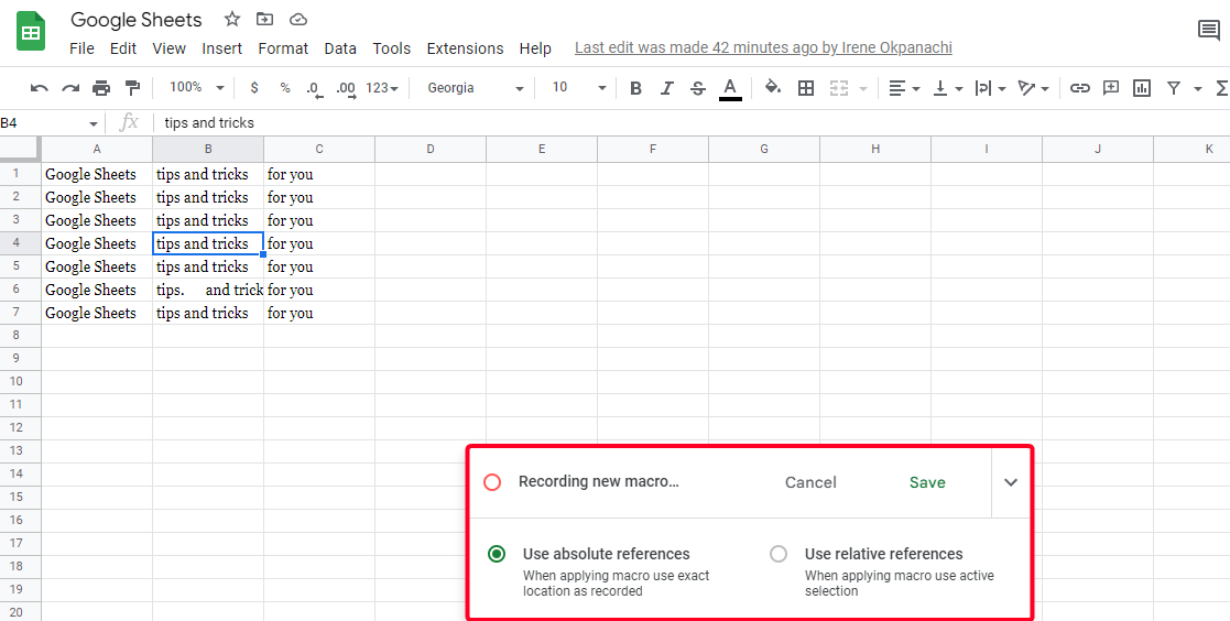
Choose a reference, then click Save.
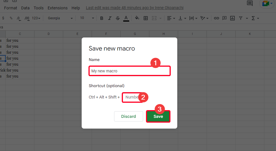
Type a name for your macro and enter a number from 0 to 9 to customize your keyboard command. Then, click Save.
To apply your macro to your spreadsheet, go to Extensions > Macros.
Select your macro, and the extension applies the macro to your spreadsheet.

Add custom functions

Google Sheets has many mathematical functions like SUM, DURATION, and FREQUENCY. If you don't find a function that does what you need, create one and add it to Sheets from the Google Apps Script extension, a platform where you can write code and integrate it with Google Workspace apps.

Apps Script is available on Google Sheets from your browser. You'll find it under the Extensions tab. The extension isn't available on the mobile app. If you're new to code, use Google Workspace Marketplace to get functions as add-ons.

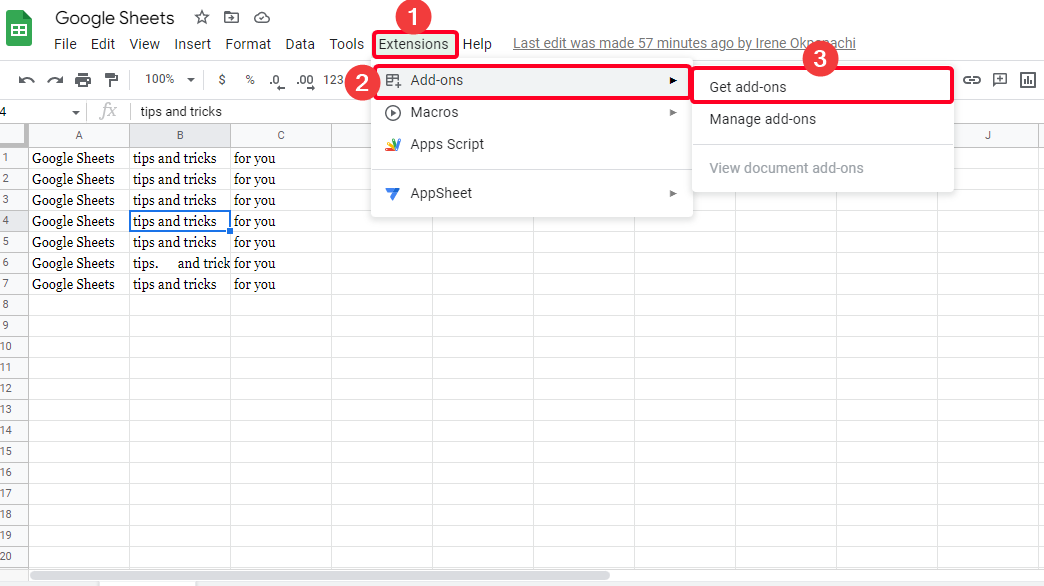
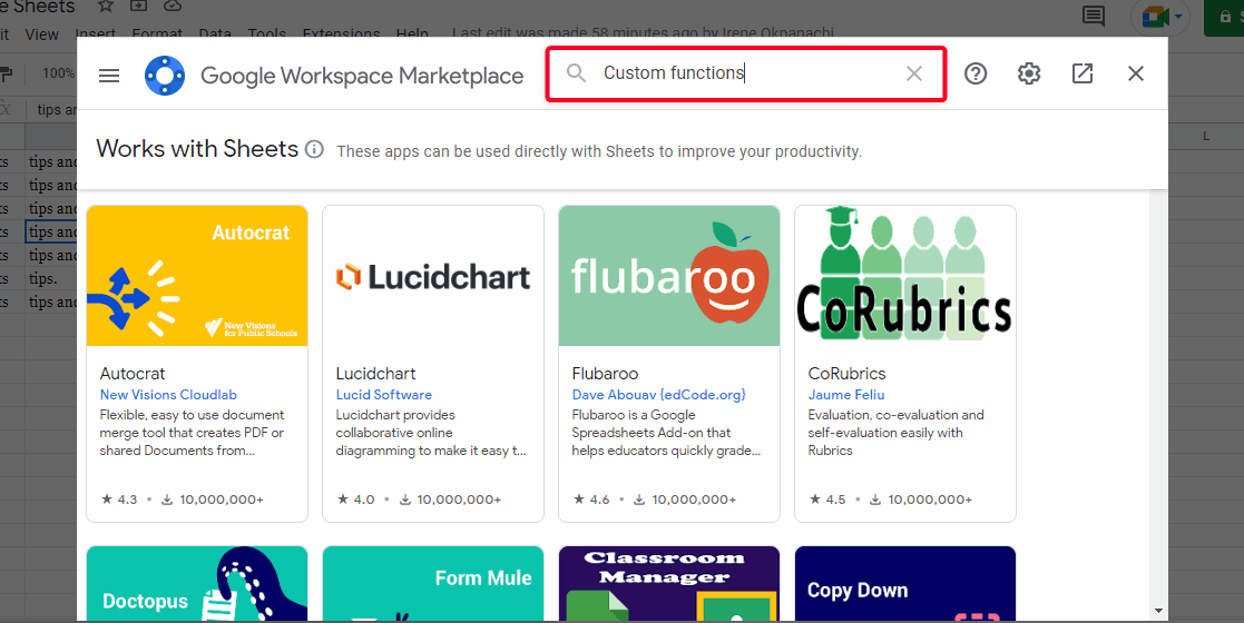
To add custom functions from Google Workspace Marketplace, go to Extensions > Add-ons > Get Add-ons.
Type Custom functions into the search bar and press the Enter key on your keyboard.
When you find a function you need, select it and click Install.
To find your new function, go to Extensions > Add-ons > Manage Add-ons.

Cleanup and trim data

Google Sheets can double-check your spreadsheet for errors. Use the cleanup tool to remove duplicate values from all or select columns. If double spaces appear between words, trim them for a neater appearance. Sheets offers suggestions on anything else that needs correcting. For example, if there are inconsistent values. This feature is not available on the mobile app.

From your browser, go to Data > Data cleanup.
To delete repeated values, click Remove duplicates.
To remove double spaces between words, click Trim whitespace.
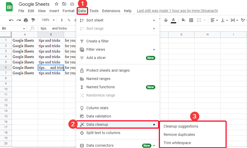
To view recommendations on what to adjust, click Cleanup suggestions. The sidebar that appears shows suggestions on what needs improvement in your spreadsheet.

Drop-down menus are useful in spreadsheets with repeated values or to collect responses in a survey. You can predefine a list of items or numbers and select from it instead of retyping the value into a cell. You can also copy and paste drop-down menus to different cells to save time.

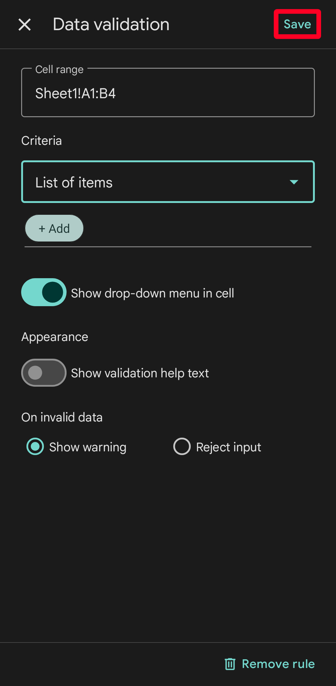
Go to Data > Data validation.
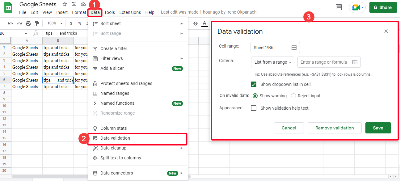
To choose where the drop-down menus appear, type a cell range.
Set the criteria for your drop-down menu.
Choose what happens when you or others select an invalid item from the list.
To let others know what your drop-down menu is for, click the Show validation help text checkbox.
Click Save. The drop-down menu appears on the spreadsheet.
To copy and paste a drop-down menu to another cell, click the cell that contains the menu.
Press Ctrl + C on your keyboard to copy the menu.
Click on the cell you want to paste it in, then press Ctrl + V on your keyboard.

Tap a cell to select it. To select multiple cells, drag the blue circle until it covers the cells you need.
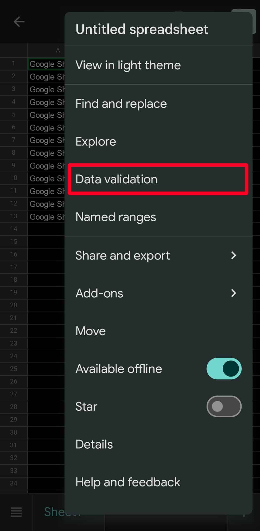
Tap the three-dot icon and select Data Validation.
Use the new menu that appears to enter a cell range, configure criteria, and edit your validation text.
Tap Save.
To copy and paste the drop-down menu to other cells, tap the cell containing the arrows. To select multiple cells, drag the blue circle to highlight them.
Long press the highlighted cells and tap Copy.
Highlight the same number of empty cells as the cells with drop-down menus.
Long press the cells and tap Paste.

Create a series

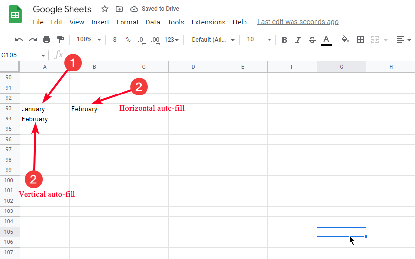
You can enter numerical values such as dates, time, whole numbers, negative numbers, and more sequentially without retyping them in Google Sheets. You can also autofill alphabets and names of months horizontally or vertically on your spreadsheet. The feature is available on the web and mobile app.

Create a series in Google Sheets on computers

Click a cell and type a value. It can be a number or the months of the year.
Go to the next cell, either horizontal or vertical to the first one.
Type the next number or month.
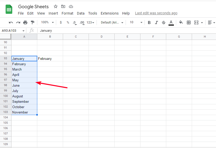
Click the first cell and drag the blue circle to the cell you want to autofill.

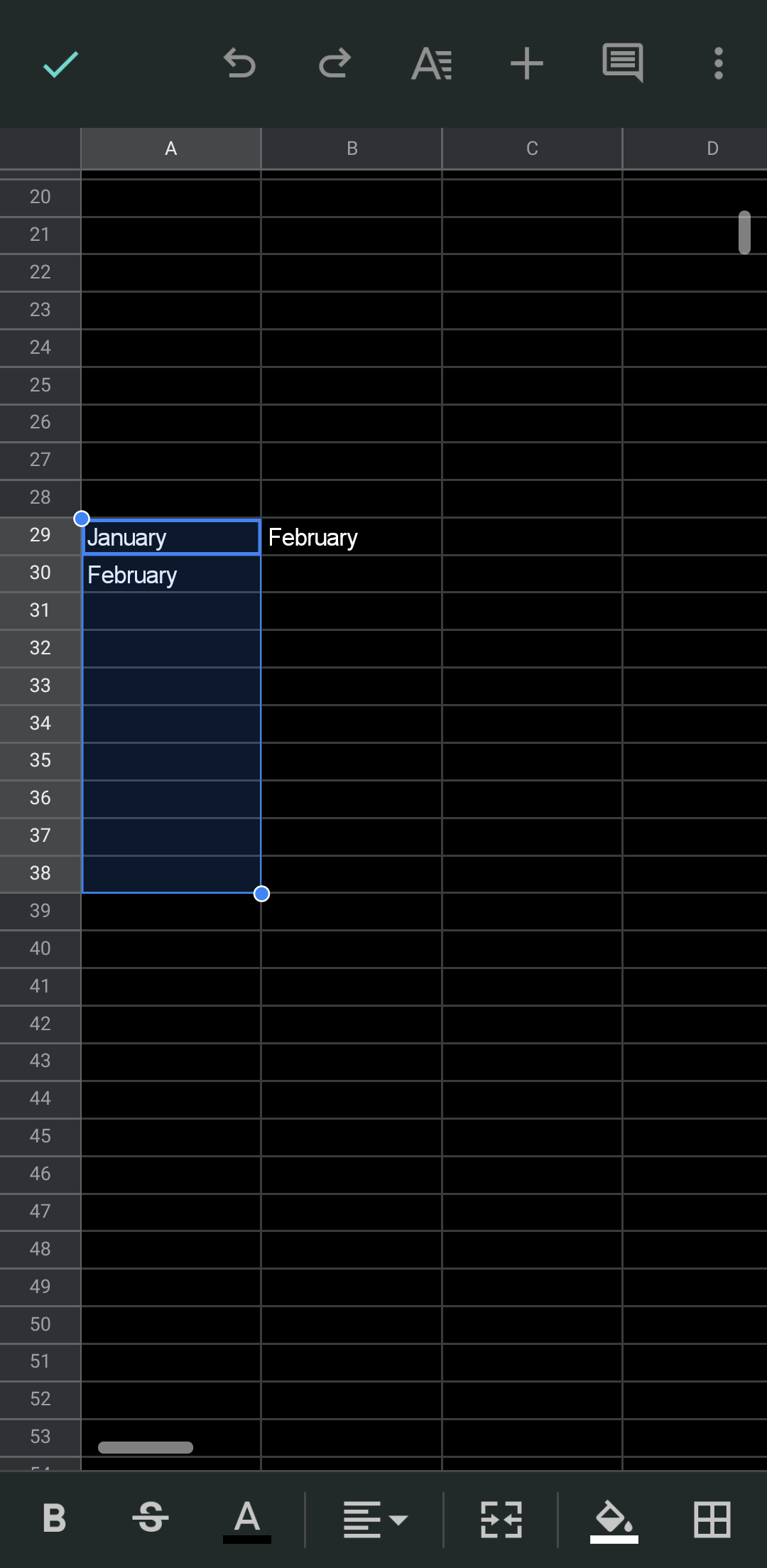
Create a series in Google Sheets on the mobile app

Tap a cell and type a value.
Go to the following cell and type the next number or letter of the value.
Tap the first cell and drag the blue circle to the cell you want to autofill.
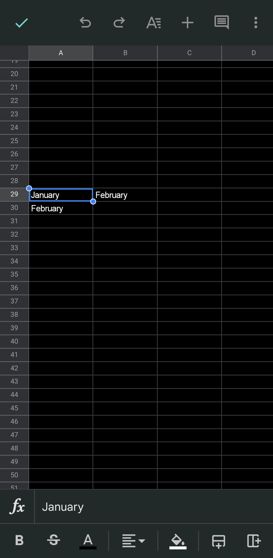
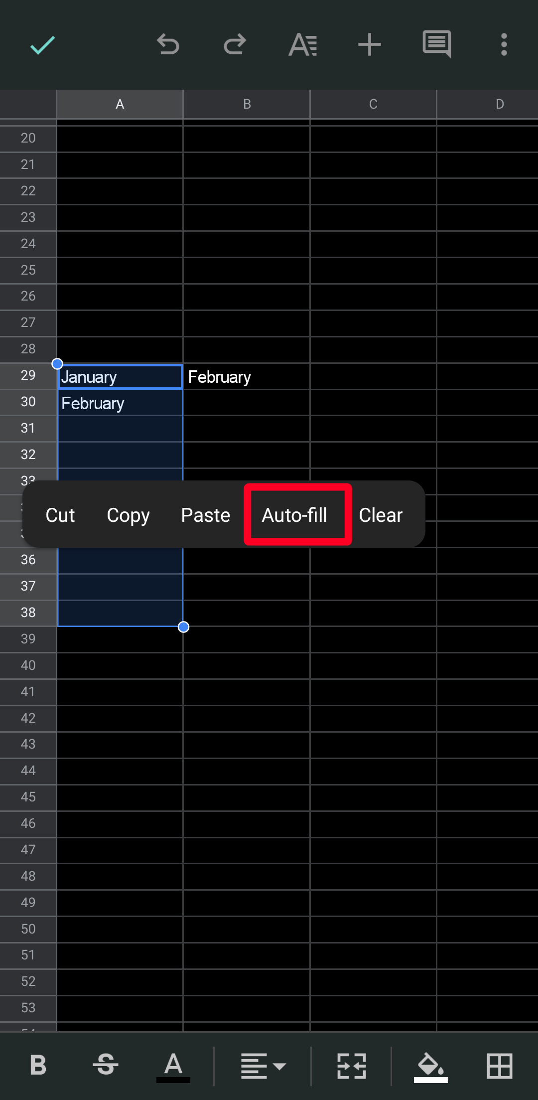
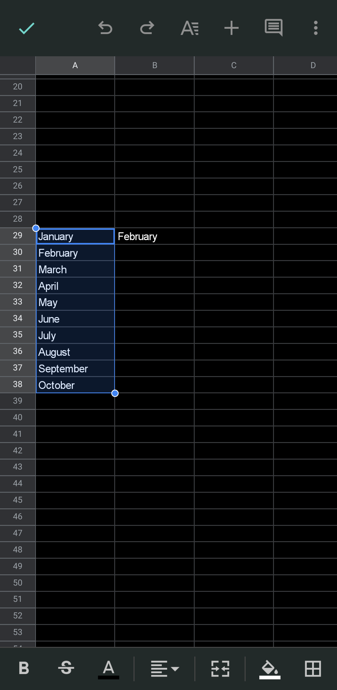
Long press the highlighted cells and tap Auto-fill.

Take data entry to the next level

Google Sheets offers powerful capabilities to simplify work. Additionally, Google Workspace Marketplace offers add-ons for your Sheets that you can use to spice up your work. You can create diagrams, build forms, make calendars and schedules, track down email addresses, generate invoices, and more.

Android Police

The top 8 Google Sheets tips and tricks that will make you more productive