Google Sheets is a powerhouse spreadsheet tool. Whether auto-suggesting formulas or fixing them for you, Sheets has all the tools you need to manage all but the most challenging spreadsheet tasks. And it's easy to use, especially if you do most of your work in the cloud and are thinking about ditching your old laptop for one of the best Chromebooks you can buy.

Sheets organizes and analyzes data to reduce the errors that come with handling large amounts of information. Large data sets are prone to duplicate data. Finding and correcting duplicate rows and cells is a painstaking task. Here's an easy way to clean up your spreadsheet and make sure you have only the data you need.

How to remove duplicate entries from Sheets

There are two ways to remove duplicates from a Sheets data set. You can use the UNIQUE function if you're comfortable working with functions. The other way is to click your way to the Data menu, which is as powerful as it is user-friendly. Both methods have strengths and weaknesses and affect your data differently.

Using UNIQUE to remove duplicate data

The biggest difference between using UNIQUE to remove redundant data and using the menu function is UNIQUE doesn't change your data set. Instead, it produces a new range of cells with the unique data.

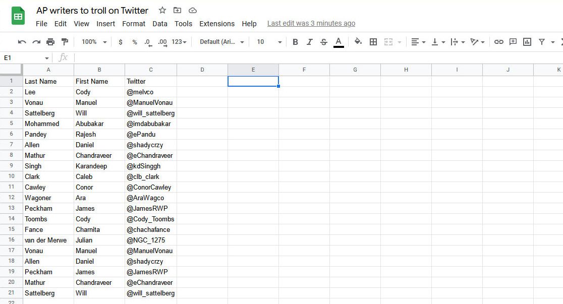
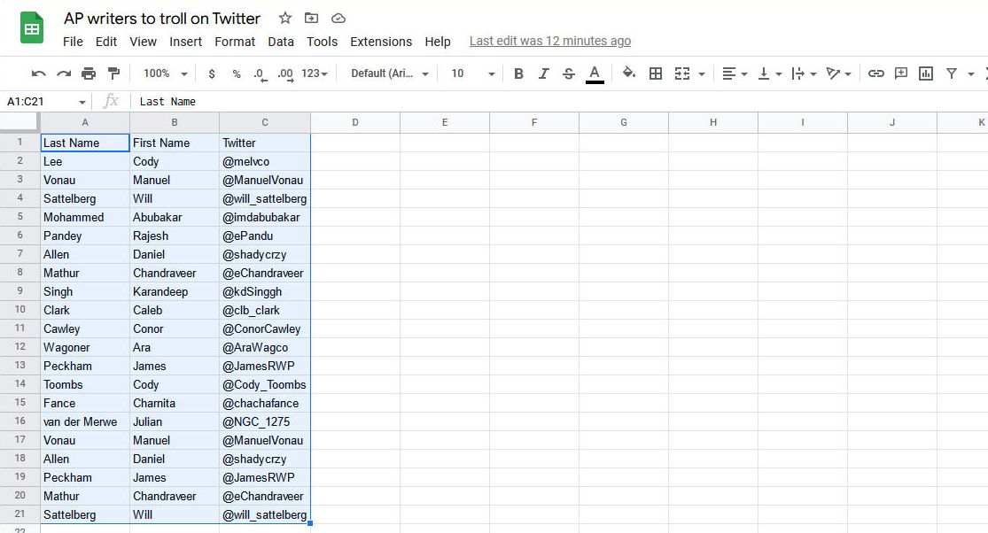
1. Highlight where you want the output of your cleaned-up data to begin. If there's not enough room to display your output, the #REF! error appears.

   

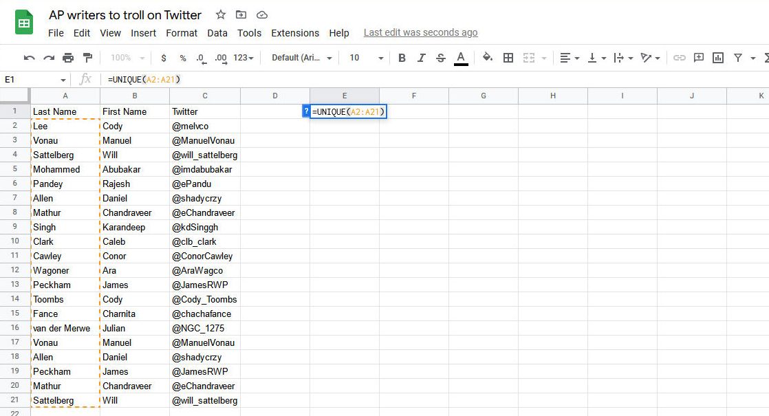
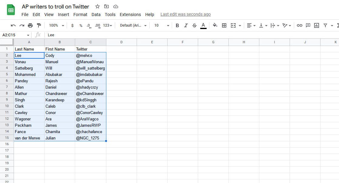
2. Type "=UNIQUE(A2:A21)" in the cell or the formula bar and adjust the range of cells based on your data. It doesn't matter if you type the function in upper case or lower case.

   

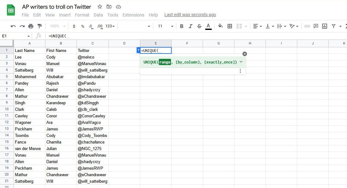
3. As you type, the pop-up help window shows the form the function should take.

   

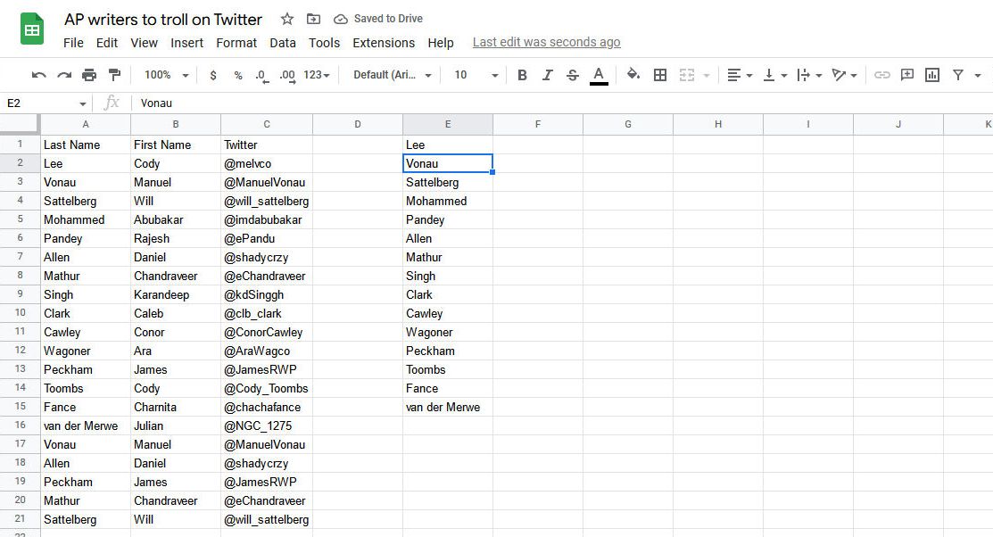
4. After typing the function, press Enter. This outputs the data from cells A2 through A21, excluding repeated data.

   

You can also use UNIQUE to modify and output more than one column of data at a time.

1. Highlight where you want the outputted data to begin.
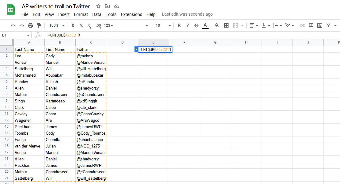
2. Type "=UNIQUE(A2:C21)" in the cell or formula bar. You'll see all three columns of data outlined.

   

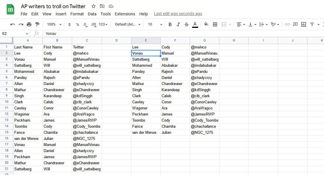
3. Press Enter. You'll see all three columns without the data that was repeated.

   

When using UNIQUE like this, it looks to see if the data in the rows are identical. In this instance, if the names are different, but the Twitter handles are the same, UNIQUE counts those rows as unique and they aren't omitted.

Where UNIQUE is superior to the Remove Duplicates function in the Data menu is its ability to work with data separated by column, not just row. The pop-up help window that appears when typing in a function shows that there's more to the UNIQUE function than a range of data. The full specification for UNIQUE looks like this:

"UNIQUE(range, [by_column], [exactly_once])"

The two bits enclosed by brackets are optional, so Sheets doesn't care if you include them. You can take advantage of these extra options by typing either true or false after the range (if you omit them, Sheets defaults their value to false).

Here's how to remove duplicates with data arranged horizontally.

1. Highlight where you want your outputted data to begin.
2. Type "=UNIQUE(B1:U3, TRUE)" and note that because "exactly_once" is optional, you don't have to write "true" or "false" in its place.

   

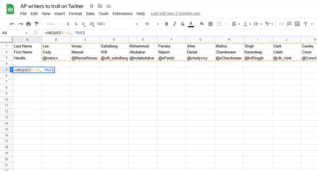
3. Press Enter.

The last optional modifier outputs only entries that appear exactly one time. The formula "=UNIQUE(A2:C21, FALSE, TRUE)" outputs a new table in which none of the names that appeared more than once would survive the cut.

One last benefit to using the UNIQUE function is that it can be combined with other functions to get you exactly the data you want, precisely how you want it organized.

Using Remove Duplicates to clear redundant data

While UNIQUE outputs new data based on a given set of cells, Remove Duplicates changes the original set of data. Here's how you use it.

1. Identify the data you want to clean up and highlight it. Make sure all the suspected duplicates are highlighted. You can highlight more columns and rows than you need.

   

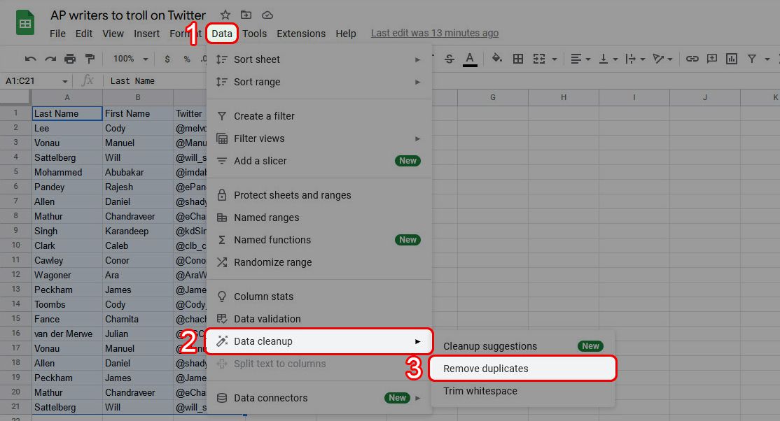
2. Go to the Data menu, hover over Data cleanup, and choose Remove duplicates.

   

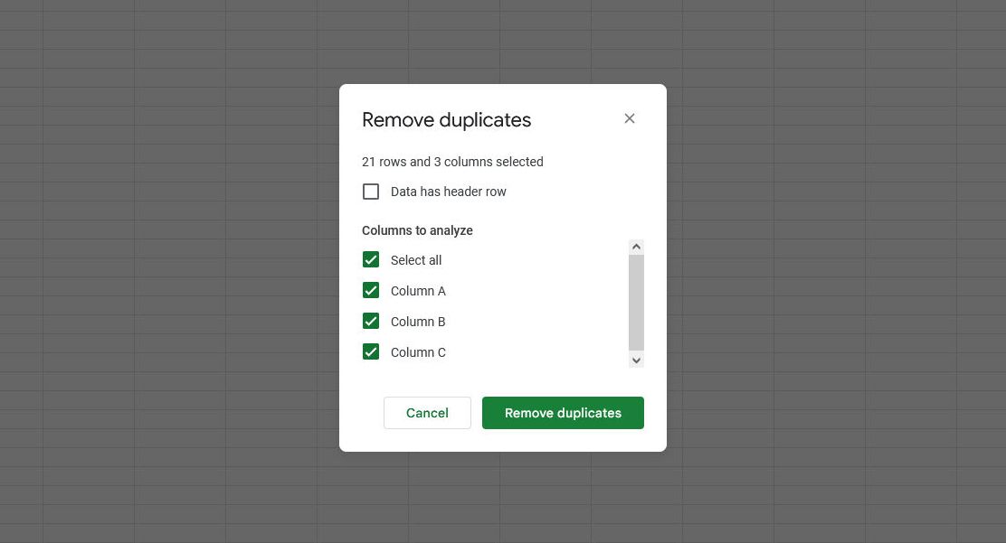
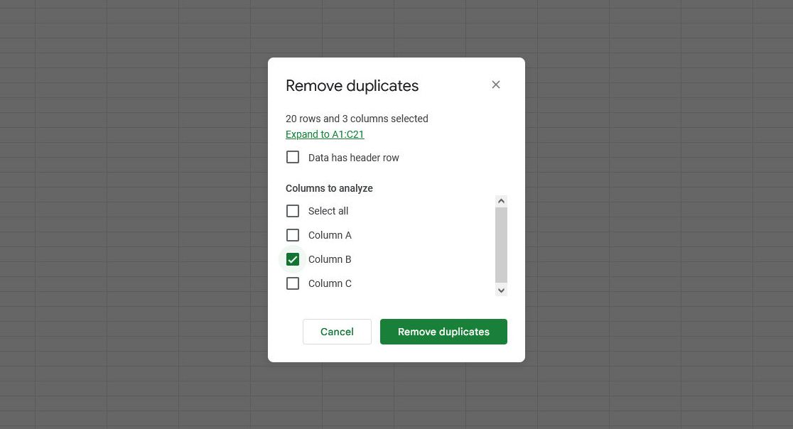
3. A new menu appears with several checkboxes where you can refine how you want Sheets to check for duplicated data. If your data has a header, select the Data has a header row checkbox. Under Columns to analyze, choose Select all.

   

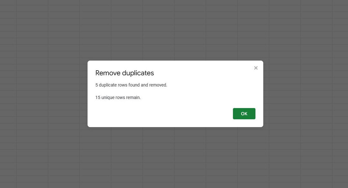
4. Click Remove duplicates. Another window pops up, telling you how many rows have been removed and how many rows remain.

   

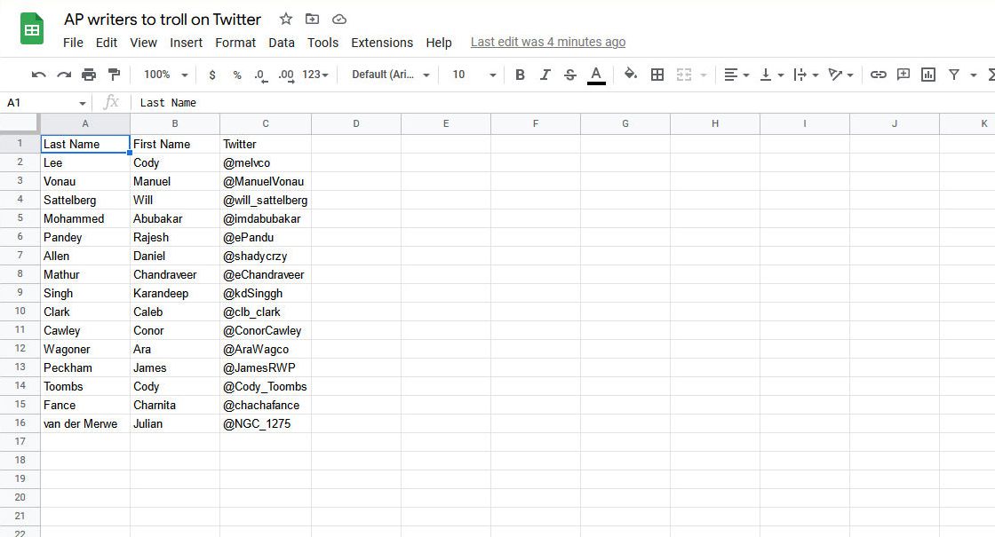
5. Click OK, and you're finished. Your data set is now clean and duplicate-free.

   

To understand what sets Remove Duplicates apart from UNIQUE, you must go back to the checkboxes that ask you which columns to analyze. Those checkboxes tell Sheets which information to check for redundancy. Here's an example to make it clearer.

1. Highlight the complete data set and navigate to Remove duplicates.
2. In the pop-up window, select only Column B under the Columns to analyze section.

   

3. Click Remove duplicates and then click OK. The previous duplicates are removed, but of the two Codys, only Cody Lee remains. Cody Toombs was cut because only the first instance of a datum is preserved (there can be only one), and all duplicate instances are cut.

   

Remove Duplicates only modifies data that's been highlighted. If you only highlight the row of last names, then none of the rows in adjacent columns are modified.

The option to analyze columns individually or as a whole gives Remove Duplicates a finer degree of control than UNIQUE. On the other hand, Remove Duplicates can only analyze data row by row, whereas UNIQUE can analyze data column by column. Given their differences in how they modify data and the difference in how they analyze them, two different tools can help you reach the same goal.

How to highlight duplicates in Google Sheets

Deleting duplicate data might not always be the best thing to do. If changing data is beyond your pay grade, the best course of action might be to highlight the duplicate data instead and let someone else figure out what to do with it. If this sounds like you, it's time to unlock the power of conditional formatting.

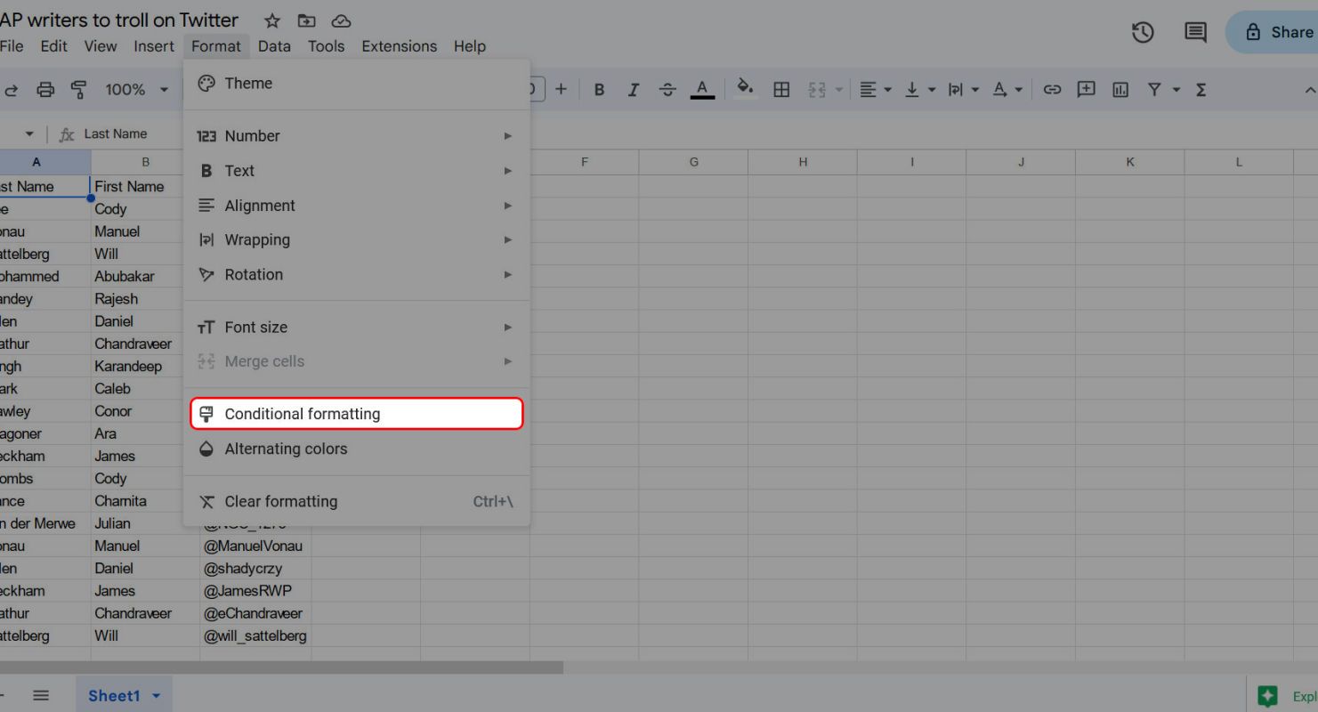
1. Click Format from the ribbon menu, then select Conditional formatting from the drop-down menu.

   

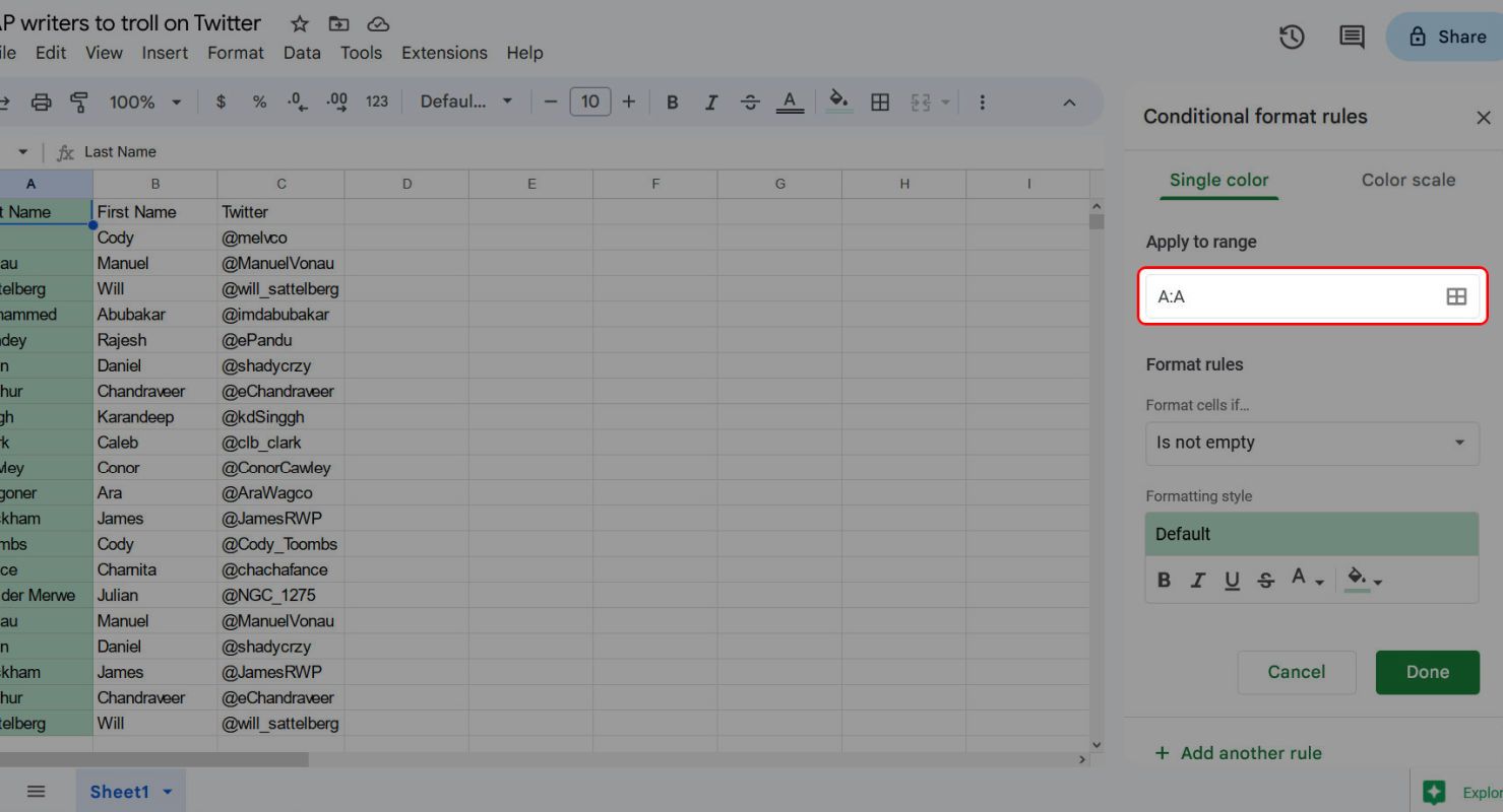
2. We're just going to work with the first column for now, so in the new pane on the right of the window, input A:A into the box that says Apply to range.

   

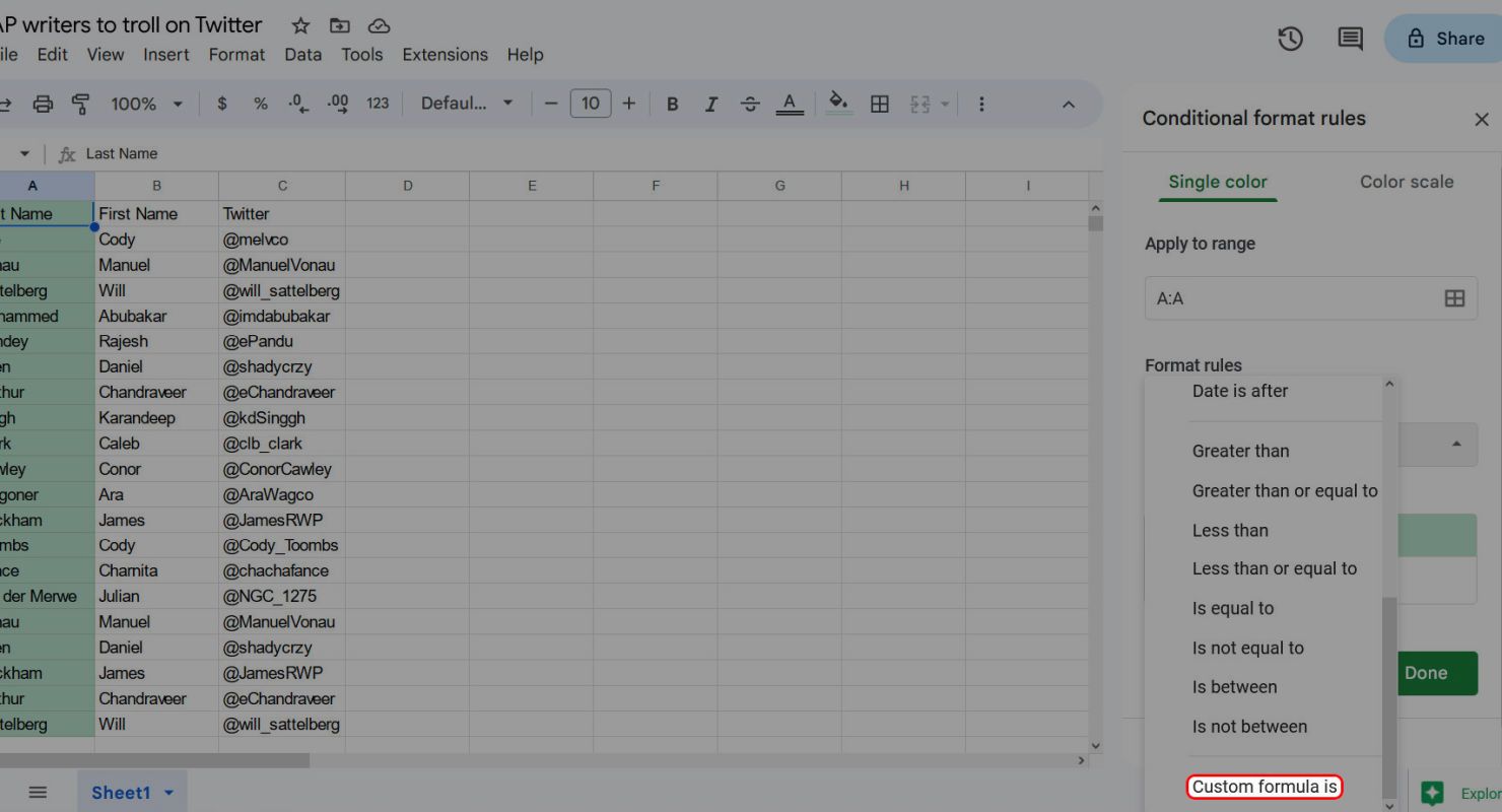
3. Under Format rules in the Format cells if drop-down menu, scroll to the bottom and select Custom formula is.

   

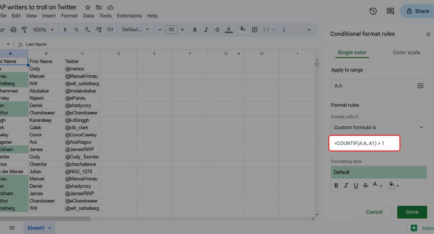
4. In the new input box that says Value or formula, enter =COUNTIF(A:A, A1) > 1. The COUNTIF function checks each cell in the range (A:A) to see if its value is repeated in another cell in the range. "A1" is a stand-in for the current value being checked. If COUNTIF finds more than one (>1) instance of that cell value, it indicates to format that particular cell.

   

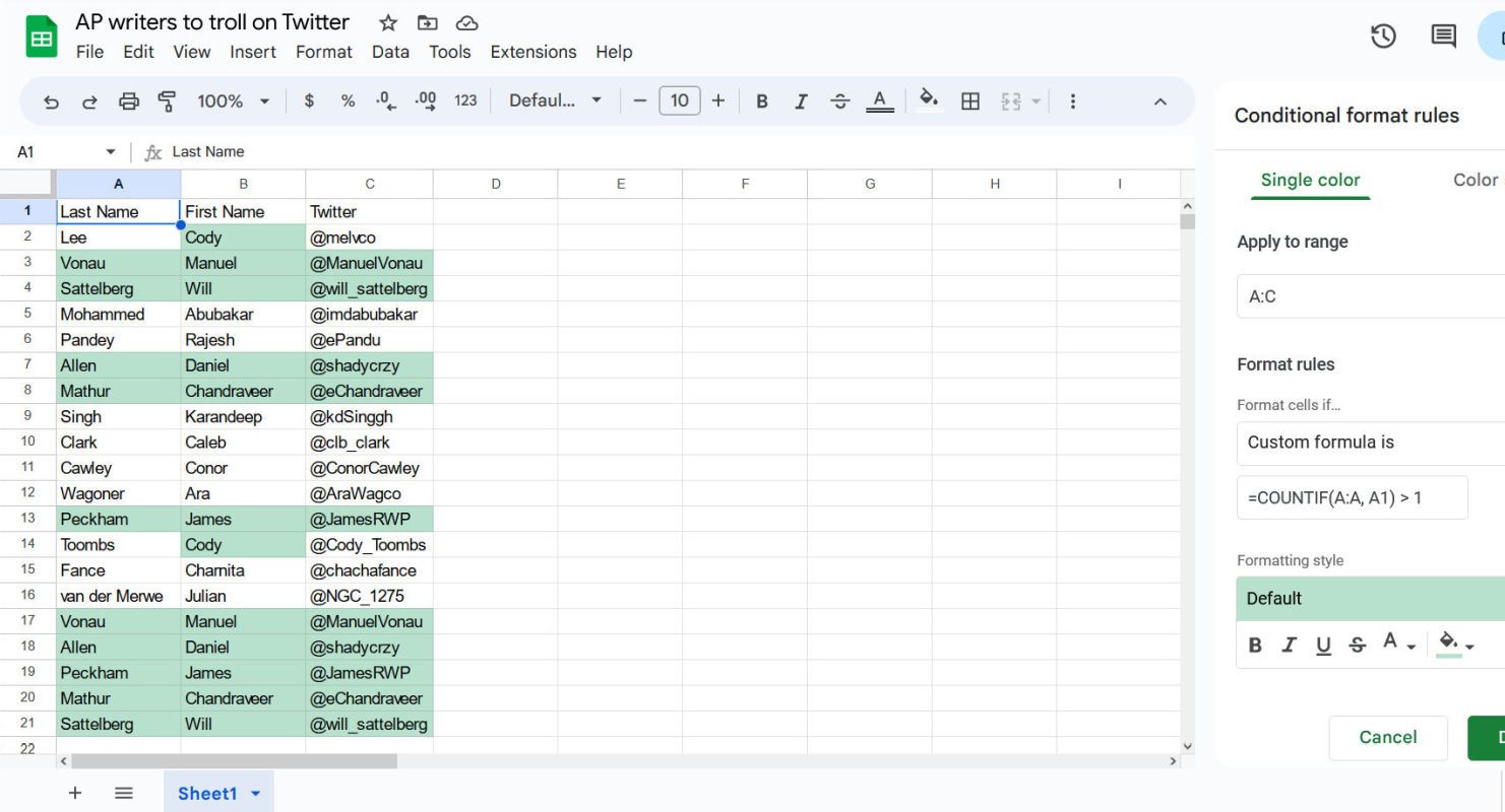
5. To expand the scope of the formatting, update the Apply to range value (let's use A:C).

   

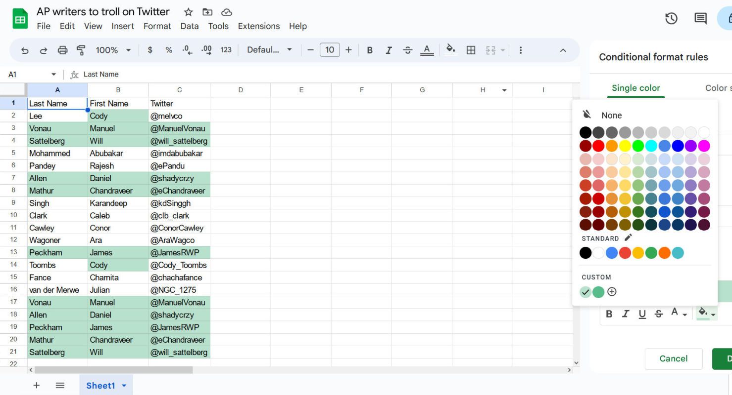
6. To change the highlight color, click the paint bucket and pick a new color.

   

Here's the result:

Start fresh with a clean worksheet

When you want to learn more about data manipulation in Google Sheets, we have guides that show you how to get rid of data, how to preserve it, and how to put it in some sort of order. Then, take a look at some of the best add-ons for Google Sheets, so even if you're not a spreadsheet wizard, you can at least pretend to be.